Orthogonale Regression

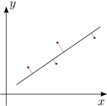
Orthogonale Regression. Die roten Linien stellen die Abstände der Messwertpaare von der Ausgleichsgeraden dar.

In der Statistik dient die orthogonale Regression (genauer: orthogonale lineare Regression) zur Berechnung einer Ausgleichsgeraden für eine endliche Menge metrisch skalierter Datenpaare ( x i , y i ) {\displaystyle (x_{i},y_{i})} nach der Methode der kleinsten Quadrate. Wie in anderen Regressionsmodellen wird dabei die Summe der quadrierten Abstände der ( x i , y i ) {\displaystyle (x_{i},y_{i})} von der Geraden minimiert. Im Unterschied zu anderen Formen der linearen Regression werden bei der orthogonalen Regression nicht die Abstände in x {\displaystyle x} - bzw. y {\displaystyle y} -Richtung verwendet, sondern die orthogonalen Abstände. Dieses Verfahren unterscheidet nicht zwischen einer unabhängigen und einer abhängigen Variablen. Damit können – anders als bei der linearen Regression – Anwendungen behandelt werden, bei denen beide Variablen x {\displaystyle x} und y {\displaystyle y} messfehlerbehaftet sind.

Die orthogonale Regression ist ein wichtiger Spezialfall der Deming-Regression. Sie wurde erstmals 1840 im Zusammenhang mit einem geodätischen Problem von Julius Weisbach angewendet[1][2], 1878 von Robert James Adcock in die Statistik eingeführt[3] und in allgemeinerem Rahmen 1943 von W. E. Deming für technische und ökonomische Anwendungen bekannt gemacht.[4]

Rechenweg

Es wird eine Gerade

y = β 0 + β 1 x {\displaystyle y=\beta _{0}+\beta _{1}x}

gesucht, die die Summe der quadrierten Abstände der ( x i , y i ) {\displaystyle (x_{i},y_{i})} von den zugehörigen Fußpunkten ( x i , y i ) {\displaystyle (x_{i}^{*},y_{i}^{*})} auf der Geraden minimiert. Wegen y i = β 0 + β 1 x i {\displaystyle y_{i}^{*}=\beta _{0}+\beta _{1}x_{i}^{*}} berechnet man diese quadrierten Abstände zu ( y i β 0 β 1 x i ) 2 + ( x i x i ) 2 {\displaystyle (y_{i}-\beta _{0}-\beta _{1}x_{i}^{*})^{2}+(x_{i}-x_{i}^{*})^{2}} , deren Summe minimiert werden soll:

S S R = i = 1 n ( ( y i β 0 β 1 x i ) 2 + ( x i x i ) 2 )     min β 0 , β 1 , x i S S R {\displaystyle SSR=\sum _{i=1}^{n}{\Big (}(y_{i}-\beta _{0}-\beta _{1}x_{i}^{*})^{2}+(x_{i}-x_{i}^{*})^{2}{\Big )}\ \to \ \min _{\beta _{0},\beta _{1},x_{i}^{*}}SSR}

Für die weitere Rechnung werden die folgenden Hilfswerte benötigt:

x ¯ = 1 n i = 1 n x i {\displaystyle {\overline {x}}={\frac {1}{n}}\sum _{i=1}^{n}x_{i}}     (arithmetisches Mittel der x i {\displaystyle x_{i}} )
y ¯ = 1 n i = 1 n y i {\displaystyle {\overline {y}}={\frac {1}{n}}\sum _{i=1}^{n}y_{i}}     (arithmetisches Mittel der y i {\displaystyle y_{i}} )
s x 2 = 1 n 1 i = 1 n ( x i x ¯ ) 2 {\displaystyle s_{x}^{2}={\tfrac {1}{n-1}}\sum _{i=1}^{n}(x_{i}-{\overline {x}})^{2}}     (Stichprobenvarianz der x i {\displaystyle x_{i}} )
s y 2 = 1 n 1 i = 1 n ( y i y ¯ ) 2 {\displaystyle s_{y}^{2}={\tfrac {1}{n-1}}\sum _{i=1}^{n}(y_{i}-{\overline {y}})^{2}}     (Stichprobenvarianz der y i {\displaystyle y_{i}} )
s x y = 1 n 1 i = 1 n ( x i x ¯ ) ( y i y ¯ ) {\displaystyle s_{xy}={\tfrac {1}{n-1}}\sum _{i=1}^{n}(x_{i}-{\overline {x}})(y_{i}-{\overline {y}})}     (Stichprobenkovarianz der ( x i , y i ) {\displaystyle (x_{i},y_{i})} )

Damit ergeben sich die Parameter zur Lösung des Minimierungsproblems:[5][6][7]

β 1 = s y 2 s x 2 + ( s y 2 s x 2 ) 2 + 4 s x y 2 2 s x y {\displaystyle \beta _{1}={\frac {s_{y}^{2}-s_{x}^{2}+{\sqrt {(s_{y}^{2}-s_{x}^{2})^{2}+4s_{xy}^{2}}}}{2s_{xy}}}}
β 0 = y ¯ β 1 x ¯ {\displaystyle \beta _{0}={\overline {y}}-\beta _{1}{\overline {x}}}

Die x {\displaystyle x} -Koordinaten der Fußpunkte berechnet man mit

x i = x i + β 1 β 1 2 + 1 ( y i β 0 β 1 x i ) {\displaystyle x_{i}^{*}=x_{i}+{\frac {\beta _{1}}{\beta _{1}^{2}+1}}(y_{i}-\beta _{0}-\beta _{1}x_{i})}

Alternativer Rechenweg

Abstand di eines Punktes P(xi;yi) zur Geraden y=mx+t

Der geometrische Abstand d i {\displaystyle d_{i}} eines Messpunktes P ( x i | y i ) {\displaystyle P(x_{i}|y_{i})} zu einer Ausgleichsgeraden

f ( x ) = m x + t {\displaystyle f(x)=mx+t}

lässt sich wegen d i : ( y i ( m x i + t ) ) = 1 : 1 + m 2 {\displaystyle d_{i}:(y_{i}-(mx_{i}+t))=1:{\sqrt {1+m^{2}}}} wie folgt berechnen:

d i 2 = ( y i ( m x i + t ) ) 2 1 + m 2 {\displaystyle d_{i}^{2}={\frac {(y_{i}-(mx_{i}+t))^{2}}{1+m^{2}}}}

Gesucht sind nun die Koeffizienten m {\displaystyle m} und t {\displaystyle t} mit der kleinsten Summe der Fehlerquadrate.

min m , t i = 1 N d i 2 {\displaystyle \min _{m,t}\sum _{i=1}^{N}d_{i}^{2}}

Berechnung der partiellen Ableitung nach t

Die Gleichung

t i = 1 N ( y i ( m x i + t ) ) 2 1 + m 2 = 0 {\displaystyle {\frac {\partial }{\partial t}}\sum _{i=1}^{N}{\frac {(y_{i}-(mx_{i}+t))^{2}}{1+m^{2}}}=0}

ergibt als Lösung

t = y ¯ m x ¯ {\displaystyle t={\overline {y}}-m{\overline {x}}}

Dabei wird als x ¯ {\displaystyle {\overline {x}}} der Mittelwert der x {\displaystyle x} -Koordinaten der Messpunkte bezeichnet. Analog dazu ist y ¯ {\displaystyle {\overline {y}}} der Mittelwert der y {\displaystyle y} -Koordinaten der Messpunkte. Diese Lösung hat auch zur Folge, dass der Punkt P ( x ¯ | y ¯ ) {\displaystyle P({\overline {x}}|{\overline {y}})} stets auf der Ausgleichsgeraden liegt.

Berechnung der partiellen Ableitung nach m

Die Gleichung

m i = 1 N ( y i ( m x i + t ) ) 2 1 + m 2 = 0 {\displaystyle {\frac {\partial }{\partial \,m}}\sum _{i=1}^{N}{\frac {(y_{i}-(mx_{i}+t))^{2}}{1+m^{2}}}=0}

ergibt folgende quadratische Gleichung:

m 2 S x y + m ( S x x S y y ) S x y = 0 {\displaystyle m^{2}S_{xy}+m(S_{xx}-S_{yy})-S_{xy}=0}

Dabei sind

S x x = i = 1 N ( x i x ¯ ) 2 {\displaystyle S_{xx}=\sum _{i=1}^{N}(x_{i}-{\overline {x}})^{2}\;} und S y y = i = 1 N ( y i y ¯ ) 2 {\displaystyle \;S_{yy}=\sum _{i=1}^{N}(y_{i}-{\overline {y}})^{2}}

die Quadratsummen der Messwerte von X {\displaystyle X} und Y {\displaystyle Y} und

S x y = i = 1 N ( x i x ¯ ) ( y i y ¯ ) {\displaystyle S_{xy}=\sum _{i=1}^{N}(x_{i}-{\overline {x}})(y_{i}-{\overline {y}})}

die Produktsumme zwischen X {\displaystyle X} und Y {\displaystyle Y} .

Auf Grund des Steigungsverhaltens dieser Parabel ergibt sich für das Minimum hier die eine Lösung:

m = S y y S x x + ( S x x S y y ) 2 + 4 ( S x y ) 2 2 S x y {\displaystyle m={\frac {S_{yy}-S_{xx}+{\sqrt {(S_{xx}-S_{yy})^{2}+4(S_{xy})^{2}}}}{2S_{xy}}}}

Die Gleichung der geometrischen Ausgleichsgeraden lautet somit:

f ( x ) = m ( x x ¯ ) + y ¯ {\displaystyle f(x)=m(x-{\overline {x}})+{\overline {y}}}

Beispiel

f(x) = 0,8 ( x – 3,3 ) + 4,1
x i {\displaystyle x_{i}} y i {\displaystyle y_{i}} x i x ¯ {\displaystyle x_{i}-{\overline {x}}} y i y ¯ {\displaystyle y_{i}-{\overline {y}}} ( x i x ¯ ) 2 {\displaystyle (x_{i}-{\overline {x}})^{2}} ( x i x ¯ ) ( y i y ¯ ) {\displaystyle (x_{i}-{\overline {x}})(y_{i}-{\overline {y}})} ( y i y ¯ ) 2 {\displaystyle (y_{i}-{\overline {y}})^{2}}
P1 1,0 2,0 −2,3 −2,1 5,29 4,83 4,41
P2 2,0 3,5 −1,3 −0,6 1,69 0,78 0,36
P3 4,0 5,0 0,7 0,9 0,49 0,63 0,81
P4 4,5 4,5 1,2 0,4 1,44 0,48 0,16
P5 5,0 5,5 1,7 1,4 2,89 2,38 1,96
Summe 16 , 5 {\displaystyle 16{,}5} 20 , 5 {\displaystyle 20{,}5} 0 , 0 {\displaystyle 0{,}0} 0 , 0 {\displaystyle 0{,}0} S x x = 11 , 8 {\displaystyle S_{xx}=11{,}8} S x y = 9 , 1 {\displaystyle S_{xy}=9{,}1} S y y = 7 , 7 {\displaystyle S_{yy}=7{,}7}
Mittelwert x ¯ = 3 , 3 {\displaystyle {\overline {x}}=3{,}3} y ¯ = 4 , 1 {\displaystyle {\overline {y}}=4{,}1}
m = 4 , 1 + 4 , 1 2 + 4 9 , 1 2 2 9 , 1 {\displaystyle m={\frac {-4{,}1+{\sqrt {4{,}1^{2}+4\cdot 9{,}1^{2}}}}{2\cdot 9{,}1}}}

Es ergibt sich m = 0 , 8 {\displaystyle m=0{,}8} und die geometrische Ausgleichsgerade lautet daher wie folgt:

f ( x ) = 0 , 8 ( x 3 , 3 ) + 4 , 1 {\displaystyle f(x)=0{,}8(x-3{,}3)+4{,}1}

Einzelnachweise

  1. J. Weisbach: Bestimmung des Hauptstreichens und Hauptfallens von Lagerstätten. In: Archiv für Mineralogie, Geognosie, Bergbau und Hüttenkunde. Band 14, 1840, S. 159–174. 
  2. D. Stoyan, T. Morel: Julius Weisbach's pioneering contribution to orthogonal linear regression. In: Historia Mathematica. Band 45, 2018, S. 75–84. 
  3. R. J. Adcock: A problem in least squares. In: The Analyst. Band 5, Nr. 2. Annals of Mathematics, 1878, S. 53–54, doi:10.2307/2635758, JSTOR:2635758. 
  4. W. E. Deming: Statistical adjustment of data. Wiley, NY (Dover Publications edition, 1985), 1943, ISBN 0-486-64685-8. 
  5. P. Glaister: Least squares revisited. The Mathematical Gazette. Vol. 85 (2001), S. 104–107.
  6. G. Casella, R. L. Berger: Statistical Inference. 2. Auflage. Cengage Learning, Boston 2008, ISBN 978-0-495-39187-6.
  7. J. Hedderich, Lothar Sachs: Angewandte Statistik. Methodensammlung mit R. 15. Auflage. Springer Berlin, Heidelberg 2015, ISBN 978-3-662-45690-3.